Build Reliable Data Workflows: SQL Techniques for Cleaning and Transforming Data

Every modern organization collects massive volumes of data—from web logs and apps to customer interactions and IoT devices. But more data doesn’t always mean more insight. The data is often messy, it may have spelling mistakes, missing values, different formats, or be spread across many sources that don’t talk to each other. On its own, this kind of data is confusing and hard to use. In fact, without structure, this information is often fragmented, inconsistent, and unusable. But when cleaned and organized, it becomes one of your most powerful tools.

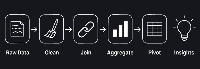
Data wrangling is the art and science of turning raw, messy, and inconsistent data into structured, reliable, and analysis-ready datasets. It involves:

• Cleaning typos, duplicates, and missing values

• Merging data from multiple sources

• Reshaping formats to suit business needs

It’s the essential first step in any meaningful data project—because no matter how advanced your models or dashboards are, they’re only as good as the data you feed them. For beginners in any data-focused role, wrangling isn’t just a technical step, it’s a critical survival skill.

SQL (Structured Query Language) is a powerful tool for data wrangling because it can efficiently handle large, structured datasets. Most companies rely heavily on SQL for data management, and it’s a standardized language across many database systems.

What You’ll Learn in This Guide

By the end of this post, you’ll be able to:

· Clean data (fixing or standardizing values using SQL functions).

• Reshape data (pivoting, aggregating retail metrics and joining tables).

• Automate data pipelines (using SQL scripts or scheduling for routine tasks).

• Perform Data quality checks (ensuring the data meets certain expectations like no nulls or out-of-range values).

Each section includes real-world SQL examples with code snippets and expected outputs to solidify these concepts. Let’s dive in!

1. Cleaning Retail Data Using SQL Functions

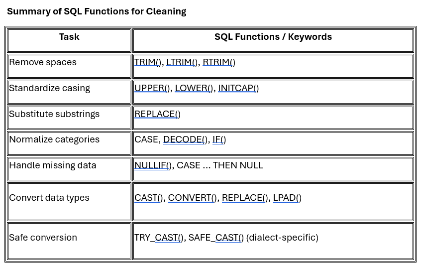
Retail datasets often arrive in messy, inconsistent formats—containing extra spaces, mixed-case labels, placeholder strings, and incorrect data types. SQL offers a comprehensive suite of functions to clean and standardize this data before analysis. Below, we break down key data cleaning categories and the associated SQL functions that should be in every data engineer or analyst’s toolkit.

1.1 Whitespace Handling

Common Issue: Product names or descriptions may contain leading or trailing spaces, leading to mismatches during filtering or joining.

Key SQL Functions:

· TRIM(column) – Removes both leading and trailing spaces (default behavior).

· LTRIM(column) – Removes leading (left) spaces only.

· RTRIM(column) – Removes trailing (right) spaces only.

Use Cases:

· Clean display names, SKUs, or textual IDs for accurate comparisons.

· Normalize data before joins or deduplication logic.

1.2 Text Standardization

Common Issue: Inconsistent casing of text values (e.g., "north", "NORTH", "North") and need for uniform labels.

Key SQL Functions:

· UPPER(column) – Converts all characters to uppercase.

· LOWER(column) – Converts all characters to lowercase.

· INITCAP(column) – Capitalizes the first letter of each word (supported in some dialects like PostgreSQL or Oracle).

· REPLACE(column, 'from', 'to') – Replaces substrings; useful for unifying spelling variations or formatting inconsistencies.

Use Cases:

· Standardize region or category names before grouping or aggregating.

· Replace problematic tokens or symbols in product attributes.

1.3 Value Normalization (Conditional Logic)

Common Issue: Labels or codes may vary for the same conceptual value (e.g., "N", "North", "NORTH").

Key SQL Constructs:

· CASE WHEN – Implements rule-based mapping and conditional recoding.

· DECODE() – Oracle-specific shortcut for CASE.

· IF() – Used in MySQL as a shorthand for binary conditional logic.

Use Cases:

· Normalize region or status codes.

· Map product categories to custom reporting groups.

· Flag invalid or suspicious entries.

1.4 Missing and Placeholder Values

Common Issue: Placeholder strings like "N/A", "Unknown", or (empty string) may be used to denote missing data.

Key SQL Functions:

· NULLIF(column, 'placeholder') – Returns NULL if column value matches the placeholder.

· CASE WHEN ... THEN NULL – More flexible logic to convert various placeholder values to proper NULL.

Use Cases:

· Convert "N/A" to NULL for compatibility with aggregate functions like AVG, COUNT, etc.

· Eliminate artificial values that break numeric summaries or affect JOIN operations.

1.5 Data Type Conversion

Common Issue: Numeric or date values may be stored as strings (e.g., "$12.99" or "2023-12-01" as VARCHAR).

Key SQL Functions:

· CAST(column AS TYPE) – Converts values to desired type (DECIMAL, DATE, INT, etc.).

· CONVERT(column, TYPE) – MySQL/T-SQL variation of CAST.

· REPLACE(column, '$', '') – Prepares string values by stripping unwanted symbols before casting.

· LPAD(column, length, pad_char) – Pads string values with leading characters (e.g., for ZIP codes).

· TRY_CAST() or SAFE_CAST() – Returns NULL instead of failing if conversion is invalid (supported in SQL Server, BigQuery, etc.).

Use Cases:

· Convert textual price or quantity fields into numeric for aggregation.

· Format ZIP codes with leading zeros.

· Safely convert date/time strings to actual DATE type.

Best Practice Patterns for SQL-Based Data Cleaning

When cleaning data with SQL, it's helpful to go beyond single-line fixes and build structured, maintainable queries. Here are three best-practice patterns you can follow—even as a beginner:

1. Stack Functions in a Single SELECT: Combine cleaning steps into one query using multiple functions.

Why it works: Compact and effective, especially when doing exploratory data analysis/profiling.

2. Use UPDATE Statements to Apply Changes Permanently: Once you're confident in your cleaning logic, apply it directly to your database.

Why it works: This keeps your database clean for everyone and not just your local analysis.

3. Use CTEs to Modularize Your Cleaning Logic: If you’re new to CTEs, think of them as “temporary, named query blocks” that you can reuse in the same query. They help break your transformations into steps, making SQL easier to debug and maintain.

Here’s what a CTE-based cleaning query looks like:

Why it works: CTEs allow you to build transformation pipelines step by step, like staging layers in a data workflow—ideal for complex cleaning tasks.

2. Reshaping Datasets with SQL: Pivoting, Aggregation, and Joins

After cleaning your data, the next major step in preparing it for analysis is reshaping—changing the structure or orientation of the data to reveal trends, compute summaries, or combine related information. SQL provides several powerful constructions to reshape data, and the most commonly used operations fall into three categories:

2.1 Pivoting: Rotating Rows to Columns

Pivoting is the process of transforming data so that unique values in a column become new columns themselves—effectively turning vertical data into a horizontal summary view.

SQL Approaches:

· PIVOT operator (supported in SQL Server, Oracle, PostgreSQL + crosstab, etc.)

· Conditional aggregation using SUM(CASE WHEN ...), supported by all SQL dialects

Use Cases:

· Converting time-series rows (e.g., months) into columns

· Generating cross-tab reports

· Comparing metrics across categories side-by-side

Scenario: You want to create a report that shows monthly sales by product category.

SQL (Portable Approach Using SUM + CASE):

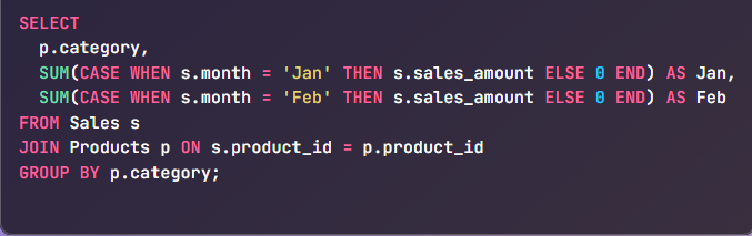
Outcome: One row per category, with separate columns for each month’s total sales.

This is a universal pivoting technique that works in all major SQL databases.

2.2 Aggregation: Summarizing Granular Data

Aggregation rolls up detailed records into summarized groups. This is essential when you're looking to derive trends or statistical summaries from raw events, transactions, logs, or sensor readings.

Common Aggregation Functions:

· SUM() – Total value

· COUNT() – Number of records

· AVG() – Average value

· MIN() / MAX() – Extremes in data

· GROUP BY – Key to grouping rows for aggregation

Use Cases:

· Computing daily or monthly totals

· Counting event types per category

· Summarizing performance metrics per department, region, or unit

Scenario: You want to calculate total and average sales per product category.

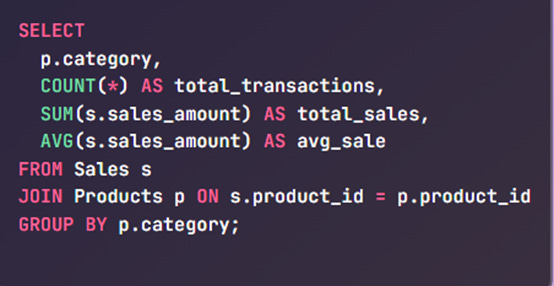
Outcome: Get meaningful KPIs like total revenue and transaction counts per category.

This structure is ideal for executive summaries and performance dashboards. Aggregations transform raw data into business-ready summaries.

2.3 Joins: Combining Data Across Tables

In most normalized databases, relevant information is distributed across multiple tables. JOINs are used to bring these fragments together into a unified dataset.

Types of Joins:

· INNER JOIN – Only matching records from both tables

· LEFT JOIN – All from the left table, and matching from the right

· RIGHT JOIN – All from the right table, and matching from the left

· FULL OUTER JOIN – All records from both sides, with NULL if no match

· CROSS JOIN – Cartesian product (rarely used in reshaping, but useful for generating combinations)

Use Cases:

· Joining transactions with user or product details

· Enriching logs with metadata

· Preparing denormalized datasets for reporting, analytics, or ML

Scenario: You want each row in your dataset to include the product name and category along with sales details.

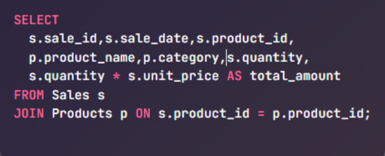
Outcome: A more readable and meaningful dataset, enriched with product context.

Joins allow you to create flattened, analysis-ready datasets from normalized tables.

Tips for Effective Reshaping in SQL

Consider using Common Table Expressions (CTEs) to modularize complex reshaping queries into readable steps.

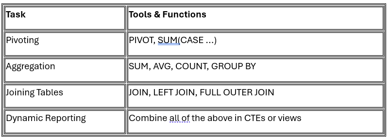
Combining Joins, Aggregations, and Pivoting: The Real-World Workflow

In production data pipelines, reshaping often requires using multiple SQL operations in a layered, sequential process. These steps allow you to transform raw, normalized tables into clean, structured outputs that power reports, dashboards, and models.

Standard Workflow Pattern:

1. JOIN all necessary tables
   Bring together your core dataset (e.g., Sales) with supporting context (e.g., Products, Stores, Customers) using keys like product_id or store_id.

2. AGGREGATE the data
   Use GROUP BY along with functions like SUM(), AVG(), COUNT() to summarize the data across meaningful dimensions (such as by product category, region, or time).

3. PIVOT the results
   Use either the PIVOT clause (in supported databases) or SUM(CASE WHEN ...) pattern to rotate categorical values (like months or regions) into columns for reporting.

Think of joins as the foundation, aggregation as the logic, and pivoting as the final presentation layer.

This multi-step approach closely reflects how data is prepared in real-world ETL (Extract, Transform, Load) pipelines. By sequentially joining, aggregating, and pivoting data, you create denormalized, analysis-ready views that are ideal for business intelligence tools, data marts, or even machine learning preprocessing. Each transformation builds on the previous one, enhancing modularity, traceability, and the overall clarity of your SQL workflows. This layered design ensures that your queries remain maintainable and scalable as data complexity grows.

3. Building Basic Automated Data Pipelines using SQL

Data wrangling isn’t a one-time affair – retail data is continuously coming in (daily sales, new products, etc.), so we often need to automate the cleaning and transformation process. A data pipeline is a series of steps to move and transform data on a schedule.

Here we’ll discuss how to implement simple pipelines using SQL scripting and scheduling, focusing on techniques like using staging tables, MERGE statements, and INSERT ... SELECT for automation.

Use Case: Imagine each day we get a CSV of the day’s online sales. We want to load it into our database daily and integrate it with a master Sales table. We can set up a pipeline:

1. Load raw data into a staging table (using a bulk load or an INSERT query).

2. Transform and merge the staging data into the main tables (using SQL transformation queries).

3. Schedule these steps to run automatically every day (using a scheduler or script).

3.1 Staging and Merging Data

Staging tables act as a buffer zone where you load incoming data, proceed to inspect or clean it, and then move it into production tables. This protects your core data from unexpected issues and helps isolate bugs.

For example:

• Sales → master table with all records.

• Sales_new → staging table for today’s batch.

The INSERT ... SELECT statement shown above simply takes all records from the Sales_new staging table and appends them to the main Sales table. After this step, the Sales table will include the new day's transactions. Depending on your needs, you might choose to empty Sales_new after processing or retain it for audit and traceability purposes.

For more advanced scenarios—such as when some records need to be updated, and others inserted—SQL provides a powerful feature called the MERGE statement (also known as an upsert). This is supported in many SQL engines and is especially useful in data warehousing workflows, where it’s common to keep dimension or fact tables continuously synchronized with new incoming data. With MERGE, you can compare records based on a key, update existing ones, and insert new ones : all in a single operation.

Example – MERGE: Let’s say we have a Products table and occasionally get updates or new products from a supplier feed. We can use a MERGE to apply these changes:

It begins by comparing records in the Product_updates table with those in the existing Products table based on the product_id. If a match is found—that is, the product already exists in the system—it updates the relevant fields, such as price and category, with the new values from the update feed. If no match is found—meaning it’s a new product—the statement inserts it as a fresh row into the Products table.

This approach ensures that your product catalog stays current, efficiently handling both updates and new entries in a single operation. In a real-world pipeline, this MERGE step would typically be scheduled to run after loading that day’s product feed into a staging table, ensuring seamless integration of new data into your system.

3.2 Automating with Scheduling

Imagine this: It's Monday morning, and your team is gathered for the weekly sales meeting. As the analyst pulls up the dashboard, everyone gasps. The numbers haven't been updated since Friday. Someone forgot to run the overnight SQL scripts again. The VP starts asking questions no one can answer, marketing campaigns launch with outdated customer segments, and the entire organization makes decisions flying blind.

This isn't just a hypothetical scenario that happens when SQL data pipelines rely on manual execution. Scheduling isn't just convenient, but critical for reliable data operations.

Schedule execution using a scheduler

• cron (Unix/Linux)

• Windows Task Scheduler

• SQL Server Agent (for MSSQL)

• BigQuery Scheduled Queries

• Apache Airflow (for more complex orchestration)

3.3 Using Temporary Tables or CTEs in Scripts

As your SQL queries become more complex, especially in analytical workflows, managing logic and readability becomes critical. Two tools that help tremendously with this are temporary tables and Common Table Expressions (CTEs).

Both are used to break down a large query into smaller, logical steps, but they serve slightly different purposes:

• Temporary tables physically store intermediate results for the duration of a session or script.

• CTEs are logical query parts—like named subqueries—that improve readability and maintainability without materializing data.

These tools help you stage, validate, and reuse data transformations in a modular and testable way—making your SQL not just functional, but scalable and understandable.

4. Implementing Simple Data Quality Checks in SQL

Once your data has been cleaned and transformed, it’s essential to ensure it meets the expected standards before it moves further down the pipeline. Data quality checks help catch issues like missing values, duplicate entries, and out-of-range figures early—before they affect dashboards, reports, or downstream systems.

Here’s how you can implement some of the most useful quality checks using SQL:

4.1 NULL or Missing Values Check

Missing values (NULLs) in key fields can lead to inaccurate analyses (e.g., sales with no product ID or orders with no customer). We can write queries to detect NULLs. For example, to check if any sales records have a null product_id or price:

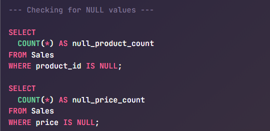
If these counts return anything other than 0, it indicates an issue. You might expect 0 missing product_ids in the Sales table (every sale should be linked to a product). Similarly, you can check other important columns.

Another approach is to pull the actual problematic rows for inspection:

This would list all sales that are incomplete. In practice, you might log these or flag them for data correction. In a pipeline, you could even fail the pipeline if critical fields are null unexpectedly.

4.2 Expected Row Counts or Uniqueness Checks

Sometimes you expect a certain number of records or unique entries. For instance, if you load daily sales, you might know approximately how many transactions occur per day (say ~10,000). You can check if the number of rows loaded is in an expected range:

If loaded_today deviates wildly from expectations (e.g., 0, or double the usual), it may indicate missing data or duplicate loading. For a stricter check, if you expect exactly one file per day, you might compare it to a control table or use a condition:

Another important check is uniqueness of key fields. If sale_id should be unique (no duplicate transactions), you can verify:

If this query returns any rows, those sale_id are duplicated (which is a data quality problem). Ideally it returns zero rows (no duplicates). Similarly, you might check that all expected product IDs from the Products table appear in the Sales table or that each store in Stores has at least one sale in Sales (depending on what business logic should hold true).

You can also perform integrity checks across tables. For example:

• Ensuring every product_id in a transaction table exists in the product catalog

• Verifying that each user action corresponds to a known user in the profile table

• Checking that every branch or store listed has at least one record in the data set

These checks help enforce business logic expectations and strengthen overall data reliability.

4.3 Value Range Enforcement

In any dataset, numeric fields often have natural boundaries—values that typically fall within a known or expected range. These can include things like non-negative quantities, realistic prices, valid age ranges, or plausible temperature readings. Detecting out-of-range values is a fundamental data quality step that helps catch input errors, upstream bugs, or pipeline glitches.

Values that are too low, too high, or logically invalid can skew aggregates, trigger incorrect alerts, or lead to poor decisions—especially if they go unnoticed.

Example: Validating Sales Values in a Retail Dataset

Let’s take a common retail dataset where each row represents a sales transaction. In such a case:

• The quantity sold should never be negative (unless returns are handled in a specific way).

• Price should be within a realistic range—likely capped based on the store’s product catalog.

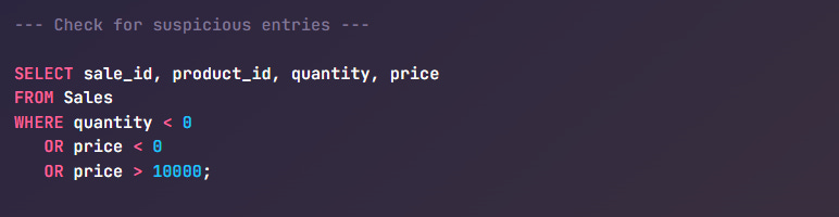
This query flags any transaction where the quantity or price seems questionable. For instance, a price greater than $10,000 might indicate a data entry error unless you're selling luxury goods. Similarly, a quantity of -5 may suggest a return that wasn’t properly categorized.

Optional: Tagging Invalid Rows

Rather than deleting bad data immediately, you can flag it for review or quarantine it in downstream processes:

This approach keeps your data traceable and gives analysts a way to exclude or investigate bad records without affecting the integrity of the raw table.

Additional Quality Checks Worth Adding

Beyond range enforcement, you can further strengthen data quality with:

• Referential Integrity Checks
  Verify that foreign key values in one table (e.g., product_id in Sales) have corresponding entries in the related reference table (e.g., Products).
  Example: Use a LEFT JOIN and filter for unmatched rows to catch orphan records.

• Consistency Checks
  Ensure internal data coherence—such as the total value in an order summary matching the sum of its line items.
  Example: Compare aggregate values across related tables (e.g., order header vs. line items).

• Timeliness Checks
  Confirm that data arrives for every expected time interval (daily, hourly, etc.), and no critical time windows are missing.
  Example: Check for missing dates in a time-series table using a calendar reference or date diff logic.

Getting Started with Data Quality Assurance

If you’re building your first SQL-based quality layer, focus on:

• NULL checks for required fields

• Duplicate detection for unique identifiers

• Range checks for numeric values

You can embed these validations directly into your data pipelines—either as QA queries after ingestion or as conditional checks that trigger alerts, logs, or even halt execution.

Doing so ensures that your datasets aren’t just updated—they’re reliable, consistent, and ready for meaningful analysis.

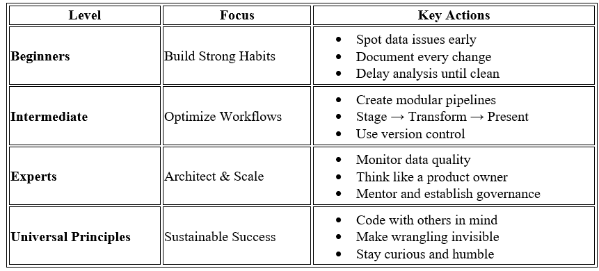
Below is quick Data Wrangling Growth Map based on your expertise level.

Key Takeaways for IT and Data Professionals

Whether you're writing ETL pipelines, managing databases, or building dashboards, SQL-based data wrangling is a foundational skill. Here’s what different roles can take away from this guide:

Data Engineers

• Learn how to clean raw, inconsistent data at scale using efficient SQL transformations.

• Apply best practices like modular CTEs, layered processing, and safe data type conversions in your data pipelines.

• Understand how to structure queries for reuse across ETL jobs and production-ready workflows.

Data Analysts / BI Developers

• Master techniques like pivoting with CASE and SUM to generate crosstab reports directly from SQL.

• Get fluent in using joins and aggregations to build report-ready datasets without waiting on upstream teams.

• Use SQL logic to standardize and reshape data before feeding it into dashboards or Excel exports.

Backend Engineers / DBAs

• Gain clarity on how to optimize and structure data for analytical workloads.

• Ensure that stored procedures and SQL views include proper cleaning and normalization steps to avoid inconsistencies.

• Apply transformations that enhance data quality and enforce business rules before data leaves the warehouse.

ML Engineers / Data Scientists

• Understand how to prepare structured data efficiently at the source, using SQL instead of excessive preprocessing in Python.

• Apply data typing, null handling, and standardization techniques that help create clean, ML-ready features.

• Reduce noise in training datasets by treating SQL cleaning as a first-class preprocessing step.

ETL & Integration Engineers

• Use this layered SQL transformation approach to build modular, maintainable ETL pipelines.

• Improve auditability by separating joins, aggregations, and pivots into distinct stages.

• Design transformations that are traceable, testable, and production-safe.

Summary

Data wrangling using SQL is a foundational capability for any data professional, particularly in dynamic sectors like retail, where data arrives from diverse sources in inconsistent formats. This tutorial explored practical techniques that help convert raw datasets into reliable, analysis-ready assets.

Proactive quality assurance mitigates downstream errors and builds organizational confidence in data-driven decision-making.

Mastering data wrangling is not merely about technical fluency in SQL—it’s about developing a mindset that values structure, clarity, and reliability. By combining robust techniques with strategic thinking, you’re not just preparing data, you’re elevating it into a trusted asset that drives business insight.

Thank You for Reading!

If this post helped you, please consider:

• Sharing it with others.

• Restacking/Bookmarking it for future reference